Insertion sort, Selection sort, bubble sort and shell sort

"INSERTION SORTING"

Insertion sort belongs to the O(n2) sorting algorithms. Unlike many sorting algorithms with quadratic complexity, it is actually applied in practice for sorting small arrays of data. For instance, it is used to improve quicksort routine. Some sources notice, that people use same algorithm ordering items, for example, hand of cards.


Algorithm
Insertion sort algorithm somewhat resembles selection sort. Array is imaginary divided into two parts - sorted one and unsorted one. At the beginning, sorted part contains first element of the array and unsorted one contains the rest. At every step, algorithm takes first element in the unsorted part and inserts it to the right place of the sorted one. When unsorted part becomes empty, algorithm stops.This will keep the left side of the array sorted until the whole array is sorted.



Example. Sort {7, -5, 2, 16, 4} using insertion sort.



Complexity analysis
Insertion sort's overall complexity is O(n2) on average, regardless of the method of insertion. On the almost sorted arrays insertion sort shows better performance, up to O(n) in case of applying insertion sort to a sorted array. Number of writes is O(n2) on average, but number of comparisons may vary depending on the insertion algorithm. It is O(n2) when shifting or swapping methods are used and O(n log n) for binary insertion sort.
From the point of view of practical application, an average complexity of the insertion sort is not so important. As it was mentioned above, insertion sort is applied to quite small data sets (from 8 to 12 elements). Therefore, first of all, a "practical performance" should be considered. In practice insertion sort outperforms most of the quadratic sorting algorithms, like selection sort or bubble sort.

"SELECTION SORTING"

Selection sort is one of the O(n2) sorting algorithms, which makes it quite inefficient for sorting large data volumes. Selection sort is notable for its programming simplicity and it can over perform other sorts in certain situations (see complexity analysis for more details).

Algorithm
The idea of algorithm is quite simple. Array is imaginary divided into two parts - sorted one and unsorted one. At the beginning, sorted part is empty, while unsorted one contains whole array. At every step, algorithm finds minimal element in the unsorted part and adds it to the end of the sorted one. When unsorted part becomes empty, algorithm stops.
When algorithm sorts an array, it swaps first element of unsorted part with minimal element and then it is included to the sorted part. This implementation of selection sort in not stable. In case of linked list is sorted, and, instead of swaps, minimal element is linked to the unsorted part, selection sort is stable.
Let us see an example of sorting an array to make the idea of selection sort clearer.
Example. Sort {5, 1, 12, -5, 16, 2, 12, 14} using selection sort.

Complexity analysis
Selection sort stops, when unsorted part becomes empty. As we know, on every step number of unsorted elements decreased by one. Therefore, selection sort makes n steps (n is number of elements in array) of outer loop, before stop. Every step of outer loop requires finding minimum in unsorted part. Summing up, n + (n - 1) + (n - 2) + ... + 1, results in O(n2) number of comparisons. Number of swaps may vary from zero (in case of sorted array) to n - 1 (in case array was sorted in reversed order), which results in O(n) number of swaps. Overall algorithm complexity is O(n2).
Fact, that selection sort requires n - 1 number of swaps at most, makes it very efficient in situations, when write operation is significantly more expensive, than read operation.

"BUBBLE SORTING"

Bubble sort is a simple and well-known sorting algorithm. It is used in practice once in a blue moon and its main application is to make an introduction to the sorting algorithms. It belongs to O(n2) sorting algorithms, which makes it quite inefficient for sorting large data volumes.It is stable and adaptive.

Algorithm
1. Compare each pair of adjacent elements from the beginning of an array and, if they are in reversed order, swap them.
2. If at least one swap has been done, repeat step 1.
You can imagine that on every step big bubbles float to the surface and stay there. At the step, when no bubble moves, sorting stops. Let us see an example of sorting an array to make the idea of bubble sort clearer.
Example. Sort {5, 1, 12, -5, 16} using bubble sort.



Complexity analysis
Average and worst case complexity of bubble sort is O(n2). Also, it makes O(n2) swaps in the worst case. Bubble sort is adaptive. It means that for almost sorted array it gives O(n) estimation. Avoid implementations, which don't check if the array is already sorted on every step (any swaps made). This check is necessary, in order to preserve adaptive property.

"SHELL SORTING"


Shell sort is the most efficient of the O(n2) class of sorting algorithms. It is also the most complex of the O(n2) algorithms. This algorithm is similar to bubble sort in the sense that it also moves elements by exchanges.
Shell sort begins by comparing elements that are at distance d. With this, the elements that are quite away from their place will move more rapidly than the simple bubble sort.
In each pass, the value of d is reduced to half.
In each pass, each element is compared with the element that is located d indexes away from it, and an exchange is made if required. The next iteration starts with a new value of d.
The algorithm terminates when d=1.

Let us consider the starting value of d to be half the number of elements. d = n/2 = 7/2 = 3

Analysis of Shell Sort
1. It is difficult to predict the complexity of Shell sort, as it is very difficult to show the effect of one pass on another pass.
2. One thing is very clear that if the new distance d is computed using the above formula, then the number of passes will approximately be log2d since d=1 will complete the sort.
3. Empirical studies have shown that the worst case complexity of Shell sort is O(n2).


To know more about sorting algorithms just click the sites below. I've also search the animation for better understanding. 

http://www.cs.oswego.edu/~mohammad/classes/csc241/samples/sort/Sort2-E.html
http://www.cs.pitt.edu/~kirk/cs1501/animations/Sort1.html
http://www.algolist.net/Algorithms/
http://www.tech-faq.com/shell-sort.html

Empirical analysis, Algorithm Analysis and The Big Oh

"EMPIRICAL ANALYSIS"

One of the branch of empirical algorithmic is the "Empirical analysis" which deals with the analysis and characterization of the behavior of  algorithm. The idea here is to consider the characteristics and performance of a certain algorithm. That is why empirical analysis is implemented in this case. there are two challenges hat we are facing in empirical analysis.First is to develop a correct and complete implementation. Basically we want to have a built-in programs that is useful to implement a complex algorithm. Second is to "determine the nature of the input data and other factors that have direct influence on the experiments to be performed". This includes all data and other properties in a an experiment. There are 3 basic choices that we are going to use: actual data, random data, or perverse data.

Actual data enable us truly to measure the cost of the program in use; random data assure us that our experiments test the algorithm, not the data; and perverse data assure us that our programs can handle any input presented them. 

Hence, there are easy steps to implement an Empirical Analysis:

1. Decide on the basic operation.-Operation which has the most running time of the algorithm-.

2. Decide on the input sample (range, size,...).data in an input sample which includes size,range,etc..

3. Convert the algorithm to a program.-converting the algorithm to a specific programming language

4. Generate a sample of inputs.-Specific sample of inputs-

5. Run the program; record the observed data. data to be observed after running the program

6. Analyze the data. -analysis of empirical data-

"ALGORITHM ANALYSIS"

What is algorithm analysis?

"Algorithm Analysis or Analysis of algorithms" is the framework for comparing algorithms and predicting performance. It also provides proof of the correctness of algorithms, allows for the accurate prediction of program performance, and can be used as a measure of computational complexity.

Why do we need to perform analysis of algorithm?

• To compare different algorithms for the same task
• To predict performance in a new environment
• To set values of algorithm parameters

  In conducting analysis of algorithm, what are we going to analyze?

In analysis of algorithm, We can:

• determine the running time of a program as a function of its inputs;
• determine the total or maximum memory space needed for program data;
• determine the total size of the program code;
• determine whether the program correctly computes the desired result;
• determine the complexity of the program--e.g., how easy is it to read, understand, and modify; and,
• determine the robustness of the program--e.g., how well does it deal with unexpected or erroneous inputs? 

 Factors that affect the running time of a program:

• the hardware:
  • processor used (type and speed),
  • memory available (cache and RAM), and
  • disk available;
• the programming language in which the algorithm is specified;
• the language compiler/interpreter used; and
• the computer operating system software. 

"BIG-Oh NOTATION"

What is Big-Oh Notation?

An O-notation, or "big-Oh notation is a mathematical artifact that allows us to suppress detail when we are analyzing algorithms. Technically speaking, it is "A function g(N) is said to be O(f(N)) if there exist constants c₀ and N₀ such that g(N) < c₀f(N) for all N > N_0".

Why do we use the O-notation?

• To bound the error that we make when we ignore small terms in mathematical formulas
• To bound the error that we make when we ignore parts of a program that contribute a small amount to the total being analyzed
• To allow us to classify algorithms according to upper bounds on their total running times

Big Oh Expressions

Concrete examples for Big-Oh Notation

*Constant time. Running time is O(1).
Elementary operations includes Function call,Boolean operation,Arithmetic operation,Assignment statement and Access array element by index.

*Logarithmic time. Running time is O (log N).
Searching in a sorted list. Given a sorted array of items, find index of query item.
O(log N) solution. Binary search.
public static int binarySearch(String[] a, String key) {
int left = 0;
int right = a.length - 1;
while (left <= right) {
int mid = left + (right - left) / 2;
int cmp = key.compareTo(a[mid]);
if (cmp < 0) right = mid - 1;
else if (cmp > 0) left = mid + 1;
else return mid;
}
return -1;
}

*Linear time. Running time is O(N).
Find the maximum. Find the maximum value of N items in an array.
double max = Double.NEGATIVE_INFINITY;
for (int i = 0; i < N; i++) {
if (a[i] > max)
max = a[i];
}

*Quadratic time. Running time is O(N ² ).
Closest pair of points. Given N points in the plane, find closest pair.
~c N2 solution. Enumerate all pairs of points.

double min = Double.POSITIVE_INFINITY;
for (int i = 0; i < N; i++){
for (int j = i+1; j < N; j++) {
double dx = (x[i] - x[j]);
double dy = (y[i] - y[j]);
if (dx*dx + dy*dy < min)
min = dx*dx + dy*dy;
}
}

*Linearithmic time. Running time is O(N log N).
Sorting. Given an array of N elements, rearrange in ascending order.
~c N log N solution. Mergesort.

*Exponential time. Running time is O(a ^N ) for some constant a > 1.
Finbonacci sequence: 1 1 2 3 5 8 13 21 34 55 …
 

public static int F(int N) {
if (n == 0 || n == 1) return n;
else return F(n-1) + F(n-2);
}

Properties of Big-Oh expressions

Complexity                                           Description                                 
 1                                 Constant algorithm is independent of input size.          

log N                            Logarithmic algorithm gets slightly slower as N        

                                     grows.

N                                 Linear algorithm is optimal if you need to process       
                                    N inputs.

N log N                       Linearithmic algorithm scales to huge problems.         

N ²                              Quadratic algorithm practical for use only on               
                                    relatively small problems.

2^N                                         Exponential algorithm is not usually practical.                

To know more about this topic, visit the following sites below.

http://www.cameron.edu/~moinian/cs3713/slide-2.6.pdf 

http://www.cs.princeton.edu/courses/archive/spr07/cos226/lectures/03Analysis.pdf

http://www.answers.com/topic/analysis-of-algorithms

http://www.answers.com/topic/empirical-algorithmics

http://www.brpreiss.com/books/opus4/html/page34.html

http://www.zanshu.com/ebook/5_algorithms-in-java-parts-1-4-third-edition/ch02lev1sec1.htm

http://www.zanshu.com/ebook/5_algorithms-in-java-parts-1-4-third-edition/ch02lev1sec2.htm

http://www.zanshu.com/ebook/5_algorithms-in-java-parts-1-4-third-edition/ch02lev1sec4.htm

UNION-FIND ALGORITHMS

UNION-FIND ALGORITHMS

A union-find algorithm is an algorithm that performs two useful operations on such a data structure: Find: Determine which group a particular element is in.
Union: Combine or merge two groups into a single group

*Quick-find solution to connectivity problem*

Sample Program implemented in java:

public class QuickF 
  { public static void main(String[] args) 
    { int N = Integer.parseInt(args[0]); 
      int id[] = new int[N]; 
      for (int i = 0; i < N ; i++) id[i] = i; 
      for( In.init(); !In.empty(); ) 
        { int p = In.getInt(), q = In.getInt(); 
          int t = id[p]; 
          if (t == id[q]) continue; 
          for (int i = 0;i<N;i++) 
            if (id[i] == t) id[i] = id[q]; 
          Out.println(" " +p+""+q); 
        } 
    } 
  } 

The program above is an implementation of a simple algorithm called the quick-find algorithm that solves the connectivity problem.

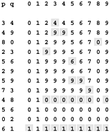
Example of quick find (slow union)

This sequence depicts the contents of the id array after each of the pairs at left is processed by the quick-find algorithm Shaded entries are those that change for the union operation. When we process the pair pq, we change all entries with the value id[p] to have the value id[q].

The quick-find algorithm executes at least MN instructions to solve a connectivity problem with N objects that involves M union operations.
For each of the M union operations, we iterate the for loop N times. Each iteration requires at least one instruction (if only to check whether the loop is finished). 

Tree representation of quick find

The connections in these figures do not necessarily represent the connections in the input. For example, the structure at the bottom has the connection 1-7, which is not in the input, but which is made because of the string of connections 7-3-4-9-5-6-1.

 

 The next algorithm that we consider is a complementary method called the quick-union algorithm. It is based on the same data structure "an array indexed by object names” but it uses a different interpretation of the values that leads to more complex abstract structures. Each object has a link to another object in the same set, in a structure with no cycles. To determine whether two objects are in the same set, we follow links for each until we reach an object that has a link to itself. The objects are in the same set if and only if this process leads them to the same object. If they are not in the same set, we wind up at different objects (which have links to themselves). To form the union, then, we just link one to the other to perform the union operation; hence the name quick union.

Tree representation of quick union

This figure is a graphical representation of the example in  Tree representation of quick find. We draw a line from object i to object id[i].

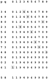
Example of quick union (not-too-quick find)

This sequence depicts the contents of the id array after each of the pairs at left are processed by the quick-union algorithm. Shaded entries are those that change for the union operation (just one per operation). When we process the pair p q, we follow links from p to get an entry i with id[i] == i; then, we follow links from q to get an entry j with id[j] == j; then, if i and j differ, we set id[i] = id[j]. For the find operation for the pair 5-8 (final line), i takes on the values 5 6901, and j takes on the values 801.

Here is the link for the union-find algorithms. all discussions are presented well. it includes all visual representation of the said algorithm. I've also searched the sample code of an algorithm. This is very helpful for our future projects. Have a nice long read!! ^_^

http://www.risc.jku.at/people/ckoutsch/stuff/e_algorithms.html
http://flylib.com/books/en/3.55.1.18/1/